Tuning a PID Controller¶

These steps apply to position PID controllers. Velocity PID controllers typically don’t need $K_d$ .

Set $K_p$ , $K_i$ , and $K_d$ to zero.
Increase $K_p$ until the output starts to oscillate around the setpoint.
Increase $K_d$ as much as possible without introducting jittering in the system response.

Plot the position setpoint, velocity setpoint, measured position, and measured velocity. The velocity setpoint can be obtained via numerical differentiation of the position setpoint (i.e., 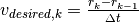$v_{desired,k} = \frac{r_k - r_{k-1}}{\Delta t}$ ). Increase $K_p$ until the position tracks well, then increase $K_d$ until the velocity tracks well.

If the controller settles at an output above or below the setpoint, one can increase $K_i$ such that the controller reaches the setpoint in a reasonable amount of time. However, a steady-state feedforward is strongly preferred over integral control (especially for PID control).

Important

Adding an integral gain to the controller is an incorrect way to eliminate steady-state error. A better approach would be to tune it with an integrator added to the plant, but this requires a model. Since we are doing output-based rather than model-based control, our only option is to add an integrator to the controller.

Beware that if $K_i$ is too large, integral windup can occur. Following a large change in setpoint, the integral term can accumulate an error larger than the maximal control input. As a result, the system overshoots and continues to increase until this accumulated error is unwound.

Note

The frc-characterization toolsuite can be used to model your system and give accurate Proportional and Derivative values. This is preferred over tuning the controller yourself.

Actuator Saturation¶

A controller calculates its output based on the error between the reference and the current state. Plant in the real world don’t have unlimited control authority available for the controller to apply. When the actuator limits are reached, the controller acts as if the gain has been termporarily reduced.

We’ll try to explain this through a bit of math. Let’s say we have a controller $u = k(r - x)$ where $u$ is the control effort, $k$ is the gain, $r$ is the reference, and $x$ is the current state. Let $u_{max}$ be the limit of the actuator’s output which is less than the uncapped value of $u$ and $k_{max}$ be the associated maximum gain. We will now compare the capped and uncapped controllers for the same reference and current state.

$u_{max} &< u \\ k_{max}(r - x) &< k(r - x) \\ k_{max} &< k$

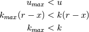
For the inequality to hold, $k_{max}$ must be less than the original value for $k$ . This reduced gain is evident in a system response when there is a linear change in state instead of an exponetial one as it approaches the reference. This is due to the control effort no longer following a decaying exponential plot. Onnce the system is closer to the reference, the controller will stop saturating and produce realistic controller values again.