Introduction to PID

The PID controller is a commonly used feedback controller consisting of proportional, integral, and derivative terms, hence the name. This article will build up the definition of a PID controller term by term while trying to provide some intuition for how each of them behaves.

First, we’ll get some nomenclature for PID controllers out of the way. The reference is called the setpoint (the desired position) and the output is called the process variable (the measured position). Below are some common variable naming conventions for relevant quantities.

\(r(t)\)	setpoint	\(u(t)\)	control input
\(e(t)\)	error	\(y(t)\)	output

The error \(e(t)\) is \(r(t) - y(t)\).

For those already familiar with PID control, this book’s interpretation won’t be consistent with the classical intuition of “past”, “present”, and “future” error. We will be approaching it from the viewpoint of modern control theory with proportional controllers applied to different physical quantities we care about. This will provide a more complete explanation of the derivative term’s behavior for constant and moving setpoints.

The proportional term drives the position error to zero, the derivative term drives the velocity error to zero, and the integral term accumulates the area between the setpoint and output plots over time (the integral of position error) and adds the current total to the control input. We’ll go into more detail on each of these.

Proportional Term

The Proportional term drives the position error to zero.

\[u(t) = K_p e(t)\]

where \(K_p\) is the proportional gain and \(e(t)\) is the error at the current time \(t\).

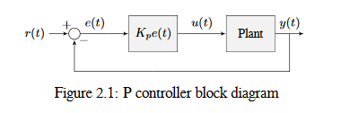
The below figure shows a block diagram for a system controlled by a P controller.

Proportional gains act like a “software-defined springs” that pull the system toward the desired position. Recall from physics that we model springs as \(F = - kx\) where \(F\) is the force applied, \(k\) is a proportional constant, and \(x\) is the displacement from the equilibrium point. This can be written another way as \(F = k(0-x)\) where \(0\) is the equilibrium point. If we let the equilibrium point be our feedback controller’s setpoint, the equations have a one to one correspondence.

\[\begin{split}F &= k(r - x) \\ u(t) &= K_p e(t) = K_p(r(t) - y(t))\end{split}\]

so the “force” with which the proportional controller pulls the system’s output toward the setpoint is proportional to the error, just like a spring.

Derivative Term

The Derivative term drives the velocity error to zero.

\[u(t) = K_p e(t) + K_d \frac{de}{dt}\]

where \(K_p\) is the proportional gain, \(K_d\) is the derivative gain, and \(e(t)\) is the error at the current time \(t\).

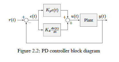
The below figure shows a block diagram for a system controlled by a PD controller.

A PD controller has a proportional controller for position (\(K_p\)) and a proportional controller for velocity (\(K_d\)). The velocity setpoint is implicitly provided by how the position setpoint changes over time. To prove this, we will rearrange the equation for a PD controller.

\[u_k = K_p e_k + K_d \frac{e_k - e_{k-1}}{dt}\]

where \(u_k\) is the control input at timestep \(k\) and \(e_k\) is the error at timestep \(k\). \(e_k\) is defined as \(e_k = r_k - x_k\) where \(r_k\) is the setpoint and \(x_k\) is the current state at timestep \(k\).

\[\begin{split}u_k &= K_p (r_k - x_k) + K_d \frac{(r_k - x_k) - (r_{k-1} - x_{k-1})}{dt} \\ u_k &= K_p (r_k - x_k) + K_d \frac{r_k - x_k - r_{k-1} + x_{k-1}}{dt} \\ u_k &= K_p (r_k - x_k) + K_d \frac{r_k - r_{k-1} - x_k + x_{k-1}}{dt} \\ u_k &= K_p (r_k - x_k) + K_d \frac{(r_k - r_{k-1}) - (x_k - x_{k-1})}{dt} \\ u_k &= K_p (r_k - x_k) + K_d \left(\frac{r_k - r_{k-1}}{dt} - \frac{x_k - x_{k-1}}{dt}\right)\end{split}\]

Notice how \(\frac{r_k - r_{k-1}}{dt}\) is the velocity of the setpoint. By the same reason, \(\frac{x_k - x_{k-1}}{dt}\) is the system’s velocity at a given timestep. That means the \(K_d\) term of the PD controller is driving the estimated velocity to the setpoint velocity.

If the setpoint is constant, the implicit velocity setpoint is zero, so the \(K_d\) term slows the system down if it’s moving. This acts like a “software-defined damper”. These are commonly seen on door closers, and their damping force increases linearly with velocity.

Integral Term

Important

Integral gain is generally not recommended for FRC® use. There are better approaches to fix steady-state error like using feedforwards or constraining when the integral control acts using other knowledge of the system.

The Integral term accumulates the area between the setpoint and output plots over time (i.e., the integral of position error) and adds the current total to the control input. Accumulating the area between two curves is called integration.

\[u(t) = K_p e(t) + K_i \int_0^t e(\tau) \,d\tau\]

where \(K_p\) is the proportional gain, \(K_i\) is the integral gain, \(e(t)\) is the error at the current time \(t\), and \(\tau\) is the integration variable.

The Integral integrates from time \(0\) to the current time \(t\). we use \(\tau\) for the integration because we need a variable to take on multiple values throughout the integral, but we can’t use \(t\) because we already defined that as the current time.

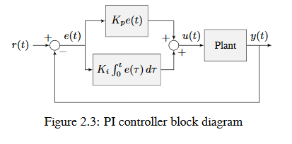
The below figure shows a block diagram for a system controlled by a PI controller.

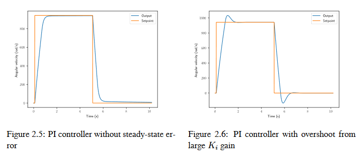
When the system is close the setpoint in steady-state, the proportional term may be too small to pull the output all the way to the setpoint, and the derivative term is zero. This can result in steady-state error as shown in figure 2.4

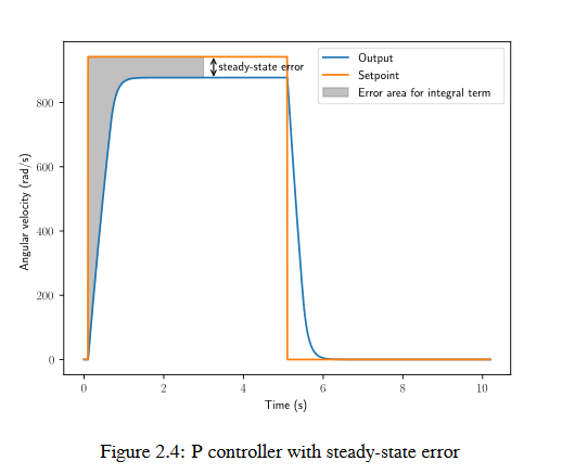
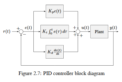
A common way of eliminating steady-state error is to integrate the error and add it to the control input. This increases the control effort until the system converges. Figure 2.4 shows an example of steady-state error for a flywheel, and figure 2.5 shows how an integrator added to the flywheel controller eliminates it. However, too high of an integral gain can lead to overshoot, as shown in figure 2.6.

PID Controller Definition

Note

For information on using the WPILib provided PIDController, see the relevant article.

When these terms are combined, one gets the typical definition for a PID controller.

\[u(t) = K_p e(t) + K_i \int_0^t e(\tau) \,d\tau + K_d \frac{de}{dt}\]

where \(K_p\) is the proportional gain, \(K_i\) is the integral gain, \(K_d\) is the derivative gain, \(e(t)\) is the error at the current time \(t\), and \(\tau\) is the integration variable.

The below figure shows a block diagram for a PID controller.

Response Types

A system driven by a PID controller generally has three types of responses: underdamped, over-damped, and critically damped. These are shown in figure 2.8.

For the step responses in figure 2.7, rise time is the time the system takes to initially reach the reference after applying the step input. Settling time is the time the system takes to settle at the reference after the step input is applied.

An underdamped response oscillates around the reference before settling. An overdamped response

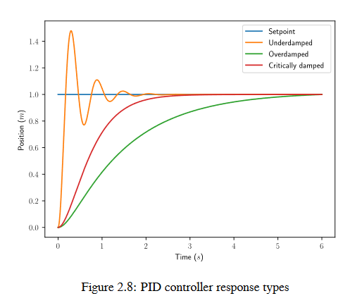
is slow to rise and does not overshoot the reference. A critically damped response has the fastest rise time without overshooting the reference.