2017 Vision Examples
LabVIEW
The 2017 LabVIEW Vision Example is included with the other LabVIEW examples. From the Splash screen, click Support->Find FRC Examples or from any other LabVIEW window, click Help->Find Examples and locate the Vision folder to find the 2017 Vision Example. The example images are bundled with the example.
C++/Java
We have provided a GRIP project and the description below, as well as the example images, bundled into a ZIP that can be found on TeamForge.
See Using Generated Code in a Robot Program for details about integrating GRIP generated code in your robot program.
The code generated by the included GRIP project will find OpenCV contours for green particles in images like the ones included in the Vision Images folder of this ZIP. From there you may wish to further process these contours to assess if they are the target. To do this:
Use the boundingRect method to draw bounding rectangles around the contours
The LabVIEW example code calculates 5 separate ratios for the target. Each of these ratios should nominally equal 1.0. To do this, it sorts the contours by size, then starting with the largest, calculates these values for every possible pair of contours that may be the target, and stops if it finds a target or returns the best pair it found.
In the formulas below, each letter refers to a coordinate of the bounding rect (H = Height, L = Left, T = Top, B = Bottom, W = Width) and the numeric subscript refers to the contour number (1 is the largest contour, 2 is the second largest, etc).
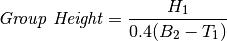
Top height should be 40% of total height (4 in / 10 in):
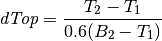
Top of bottom stripe to top of top stripe should be 60% of total height (6 in / 10 in):
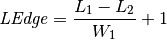
The distance between the left edge of contour 1 and the left edge of contour 2 should be small relative to the width of the 1st contour; then we add 1 to make the ratio centered on 1:
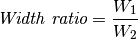
The widths of both contours should be about the same:
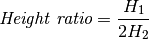
The larger stripe should be twice as tall as the smaller one
Each of these ratios is then turned into a 0-100 score by calculating:

To determine distance, measure pixels from top of top bounding box to bottom of bottom bounding box:
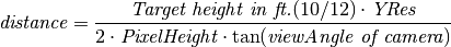
The LabVIEW example uses height as the edges of the round target are the most prone to noise in detection (as the angle points further from the camera the color looks less green). The downside of this is that the pixel height of the target in the image is affected by perspective distortion from the angle of the camera. Possible fixes include:
Try using width instead
Empirically measure height at various distances and create a lookup table or regression function
Mount the camera to a servo, center the target vertically in the image and use servo angle for distance calculation (you’ll have to work out the proper trig yourself or find a math teacher to help!)
Correct for the perspective distortion using OpenCV. To do this you will need to calibrate your camera with OpenCV. This will result in a distortion matrix and camera matrix. You will take these two matrices and use them with the undistortPoints function to map the points you want to measure for the distance calculation to the “correct” coordinates (this is much less CPU intensive than undistorting the whole image)