状态观察者和卡尔曼滤波器
状态观察者将关于系统行为的信息和外部度量结合起来,以估计系统的真实状态。线性系统常用的观测器是卡尔曼滤波器。卡尔曼滤波器比其他 :ref:`filters <docs/software/advanced-controls/filters/index:Filters>`更有优势,因为它们将来自一个或多个传感器的测量结果与系统的状态空间模型相融合,以最佳估计系统的状态。
这张图片显示了飞轮速度随时间的测量,通过各种不同的过滤器运行。注意,一个调谐良好的卡尔曼滤波器在飞轮旋转时没有显示测量滞后,同时仍然拒绝噪声数据,并对球通过时的干扰做出快速反应。更多关于过滤器的信息可以在:ref:filters section <docs/software/advanced-controls/filters/index:Filters>找到。

高斯函数
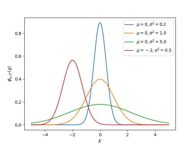
Kalman filters utilize a Gaussian distribution to model the noise in a process [1]. In the case of a Kalman filter, the estimated state of the system is the mean, while the variance is a measure of how certain (or uncertain) the filter is about the true state.
方差和协方差的概念是卡尔曼滤波器功能的核心。协方差是对两个随机变量相关程度的度量。在一个只有一个状态的系统中,协方差矩阵就是简单的:math:mathbf{text{cov}(x_1, x_1)},或者是一个包含状态 \(x_1`的方差:math:\)mathbf{text{var}(x_1)}` 的矩阵。该方差的大小是描述当前状态估计的高斯函数的标准差的平方。协方差相对较大的值可能表示有噪声的数据,而较小的协方差可能表示过滤器对它的估计更有信心。记住,方差或协方差的“大”值和“小”值与所使用的基本单位有关——例如,如果:math:mathbf{x_1}`是以米计量,:math:mathbf{text{cov}(x_1, x_1)}` 将以米的平方计量。
协方差矩阵可写成如下形式:
卡尔曼滤波器
重要
对卡尔曼滤波器的实际作用有一个直观的认识是很重要的。`Kalman and Bayesian Filters in Python by Roger Labbe <https://github.com/rlabbe/Kalman-and-Bayesian-Filters-in-Python>`一书提供了贝叶斯滤波器极佳的可视化和互动性介绍。WPILib中的卡尔曼滤波器使用线性代数来美化数学,但其思想与一维情况相似。我们建议通读第4章,直观了解这些过滤器在做什么
To summarize, Kalman filters (and all Bayesian filters) have two parts: prediction and correction. Prediction projects our state estimate forward in time according to our system’s dynamics, and correct steers the estimated state towards the measured state. While filters often perform both in the same timestep, it’s not strictly necessary – For example, WPILib’s pose estimators call predict frequently, and correct only when new measurement data is available (for example, from a low-framerate vision system).
下面给出了离散时间卡尔曼滤波器的方程:
状态估计 \(\mathbf{x}`和 :math:\)mathbf{P}`’描述高斯函数的均值和协方差,高斯函数描述了我们的滤波器对系统真实状态的估计。
处理和测量噪声协方差矩阵
过程和测量噪声协方差矩阵:math:mathbf{Q} 和 \(\mathbf{R}\) 描述了我们的每个状态和测量的方差。记住,对于高斯函数,方差是函数标准差的平方。在WPILib中,Q和R是对角矩阵,它们的对角线包含各自的方差。例如,卡尔曼滤波状态 \(\begin{bmatrix}\text{position} \\ \text{velocity} \end{bmatrix}\) 和具有状态标准差 \(\begin{bmatrix}0.1 \\ 1.0\end{bmatrix}\) 和测量标准差 \(\begin{bmatrix}0.01\end{bmatrix}\) 的测量 \(\begin{bmatrix}\text{position} \end{bmatrix}\) 将具有下面的:math:mathbf{Q} 和 \(\mathbf{R}\) 矩阵:
误差协方差矩阵
误差协方差矩阵 \(\mathbf{P}`描述了状态估计的协方差:math:\)mathbf{hat{x}}`。非正式地,\(\mathbf{P}\) 描述了我们对估计 state`的确定性。如果 :math:mathbf{P}`很大,真实状态的不确定性就很大。相反,元素更小的:math:`mathbf{P}`意味着我们真实状态的不确定性更小。
当我们向前预测模型时,\(\mathbf{P}\) 会随着我们对系统真实状态的确定性降低而增加。
预测步骤
在预测中,我们的状态估计是根据线性系统动力学:math:mathbf{dot{x} = Ax + Bu}`更新的。此外,我们的误差协方差:math:mathbf{P}` 随着过程噪声协方差矩阵:math:mathbf{Q}`的增大而增大,:math:mathbf{Q}`的值越大,我们的误差协方差 \(\mathbf{P}\) 增长得越快。这个 \(\mathbf{P}\) 用于校正步骤,以权重模型和测量。
校正步骤
在校正步骤中,我们的状态估计值将更新为包含新的测量信息。这个新信息通过卡尔曼增益 \(\mathbf{K}`与状态估计值:math:\)mathbf{hat{x}}`进行加权,较大的 \(\mathbf{K}\).值对进入测量值的权重更高,较小的 \(\mathbf{K}\) 值对我们的状态预测的权重更高。因为 \(\mathbf{K}`与 :math:\)mathbf{P}`相关, \(\mathbf{P}`值越大, :math:\)mathbf{K}`就越高,重量测量也越重。例如,如果一个过滤器预测了很长一段时间,那么大的:math:`mathbf{P}`将会赋予新信息很大的权重。
最后,误差协方差 \(\mathbf{P}\) 减少,以增加我们对状态估计的信心。
调整卡尔曼过滤器
WPILib的卡尔曼滤波类的构造器采用线性系统、过程噪声标准差和测量噪声标准差向量。通过用每个状态或测量的标准差或方差的平方填充对角线,这些矩阵转换为:math:mathbf{Q} 和 \(\mathbf{R}`矩阵。通过减少一个状态的标准偏差(以及:math:\)mathbf{Q}`中相应的条目),过滤器将更加不信任传入的度量。类似地,增加一个州的标准偏差将更信任传入的测量结果。对于测量标准偏差也是如此——减少一个条目将使过滤器更加信任输入的测量值对应的状态,而增加它将降低对测量值的信任。
48  // The observer fuses our encoder data and voltage inputs to reject noise.
49  private final KalmanFilter<N1, N1, N1> m_observer =
50      new KalmanFilter<>(
51          Nat.N1(),
52          Nat.N1(),
53          m_flywheelPlant,
54          VecBuilder.fill(3.0), // How accurate we think our model is
55          VecBuilder.fill(0.01), // How accurate we think our encoder
56          // data is
57          0.020);
 5#include <numbers>
 6
 7#include <frc/DriverStation.h>
 8#include <frc/Encoder.h>
 9#include <frc/TimedRobot.h>
10#include <frc/XboxController.h>
11#include <frc/controller/LinearQuadraticRegulator.h>
12#include <frc/drive/DifferentialDrive.h>
13#include <frc/estimator/KalmanFilter.h>
14#include <frc/motorcontrol/PWMSparkMax.h>
15#include <frc/system/LinearSystemLoop.h>
16#include <frc/system/plant/DCMotor.h>
17#include <frc/system/plant/LinearSystemId.h>
18#include <units/angular_velocity.h>
48  // The observer fuses our encoder data and voltage inputs to reject noise.
49  frc::KalmanFilter<1, 1, 1> m_observer{
50      m_flywheelPlant,
51      {3.0},   // How accurate we think our model is
52      {0.01},  // How accurate we think our encoder data is
53      20_ms};
48        # The observer fuses our encoder data and voltage inputs to reject noise.
49        self.observer = wpimath.estimator.KalmanFilter_1_1_1(
50            self.flywheelPlant,
51            [3],  # How accurate we think our model is
52            [0.01],  # How accurate we think our encoder data is
53            0.020,
54        )